[Example 1] Simple curved channel with a 60 degree bend
Select a solver
From the [Select Solver] window, select [Nys2d+] and click [OK].
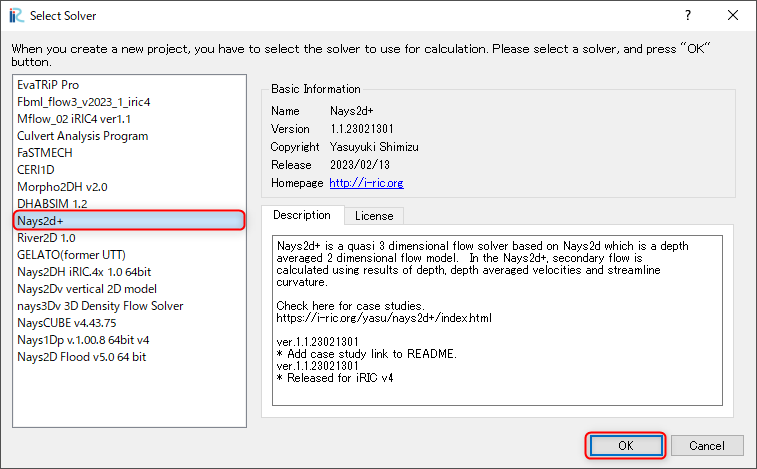
Figure 4 : Select Solver
A window with [Untitled - iRIC 3.x.xxxx [Nays2d+]] appears.
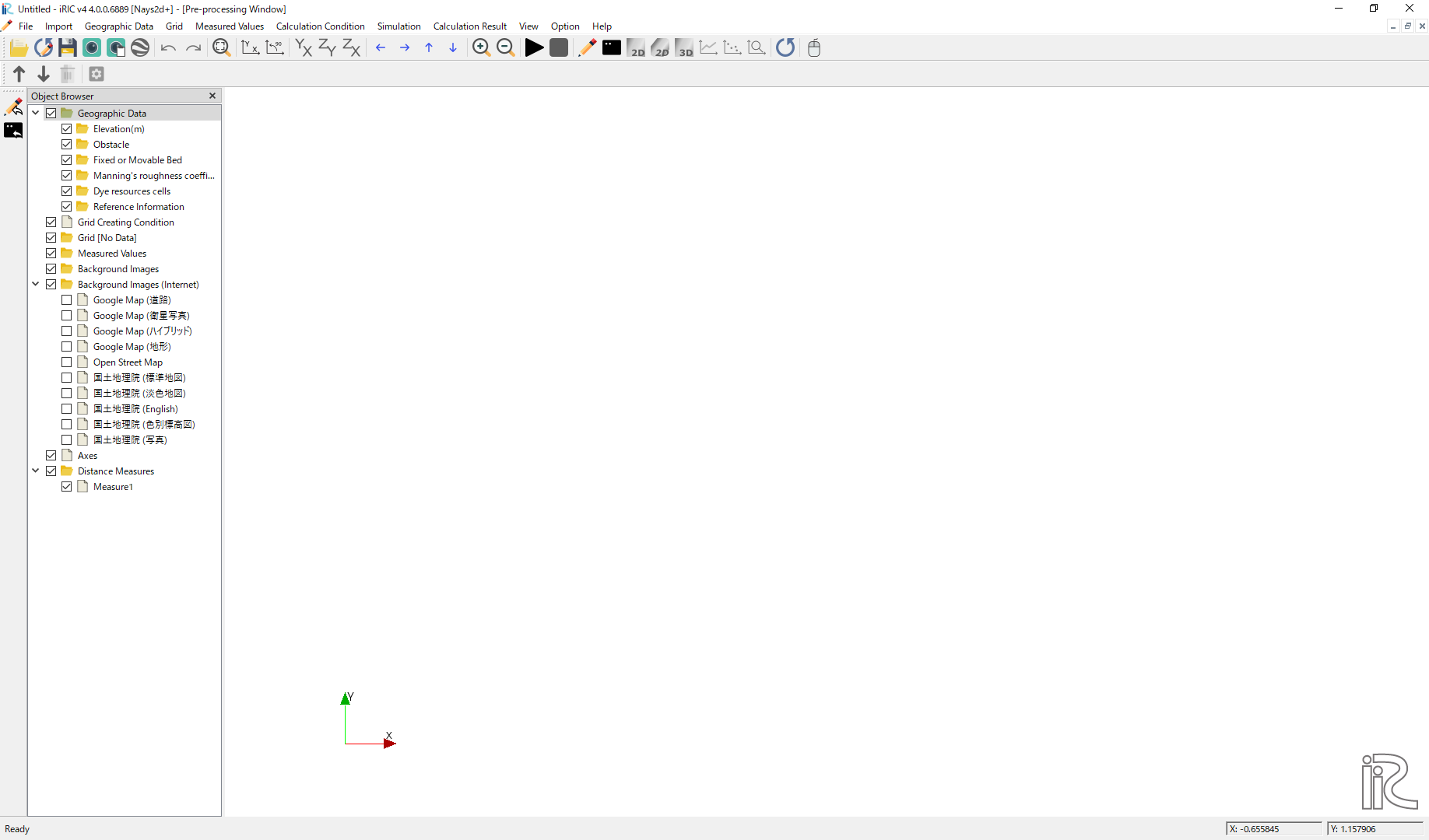
Figure 5 : Untitled
From the window, Figure 5 ,select [Grid], [Select Algorithm to Create Grid]. Then the [Select Grid Creating Algorithm] window, Figure 7 appears.
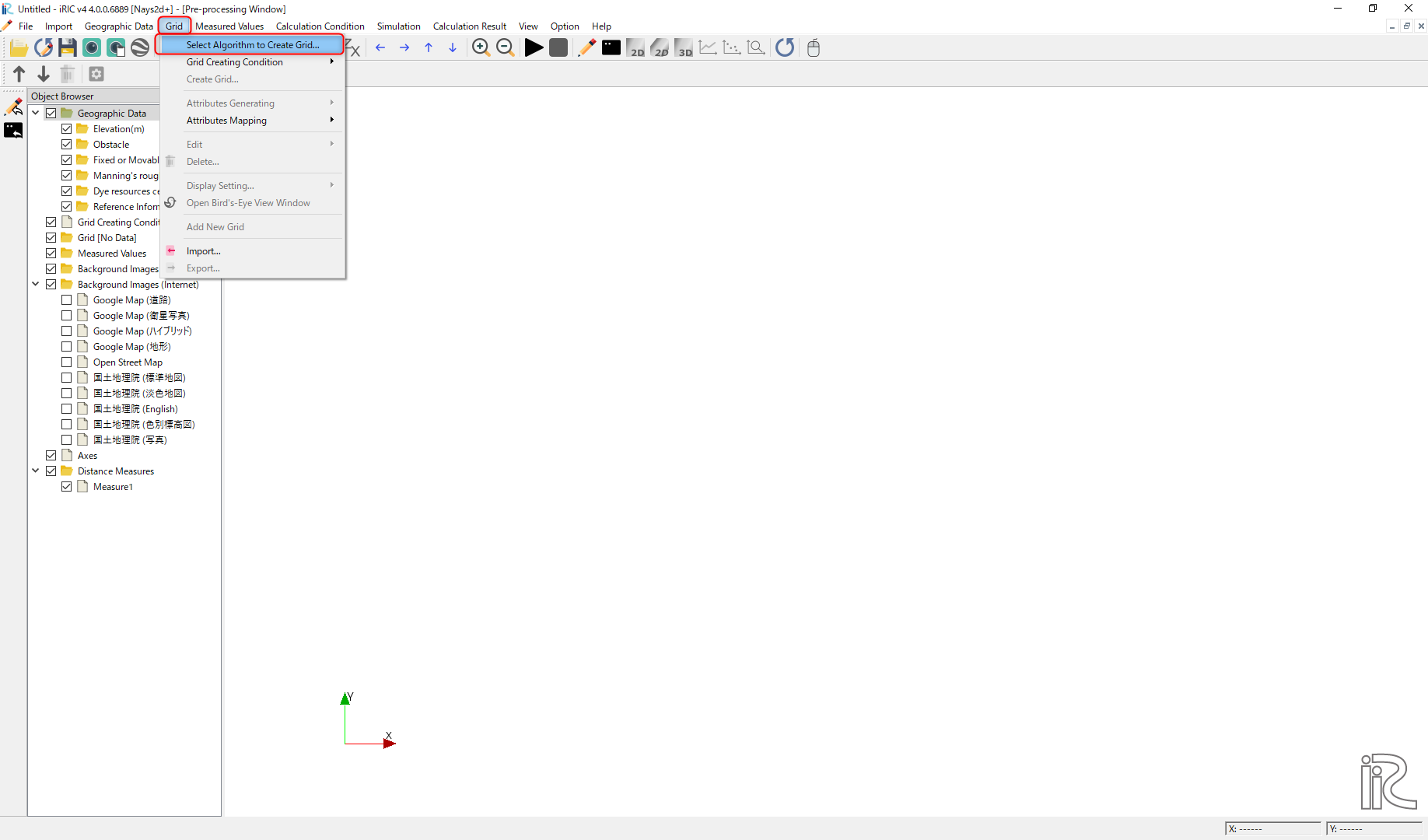
Figure 6 : Select Algorithm t Create Grid
Select [2d arc grid generator], and push [OK]
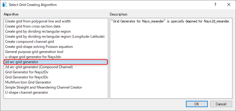
Figure 7 : Select Grid Creating Algorithm
Create Computational Grid
In the window, Figure 8 , click [Channel shape (basic)], and set the values as show in Figure 8 .
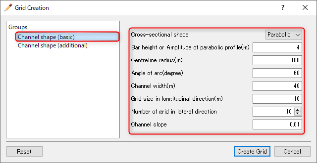
Figure 8 :Channel shape (basic)
Select [Channel shape (additional)], set the values as shown in Figure 9 , and click [Create Grid].
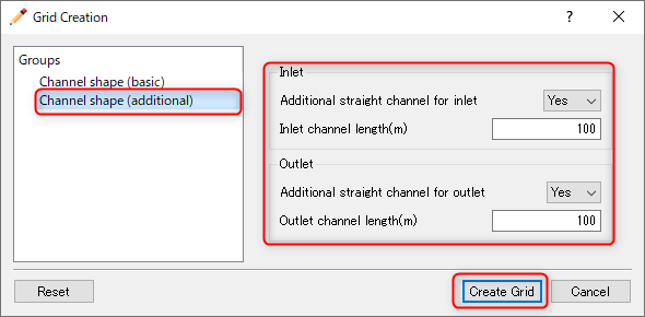
Figure 9 :Channel shape (additional)
Then the [Conformation] window appears as Figure 10 ,and click [Yes].
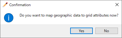
Figure 10 :Confirmation for mapping
Then the following window, Figure 11 appears.
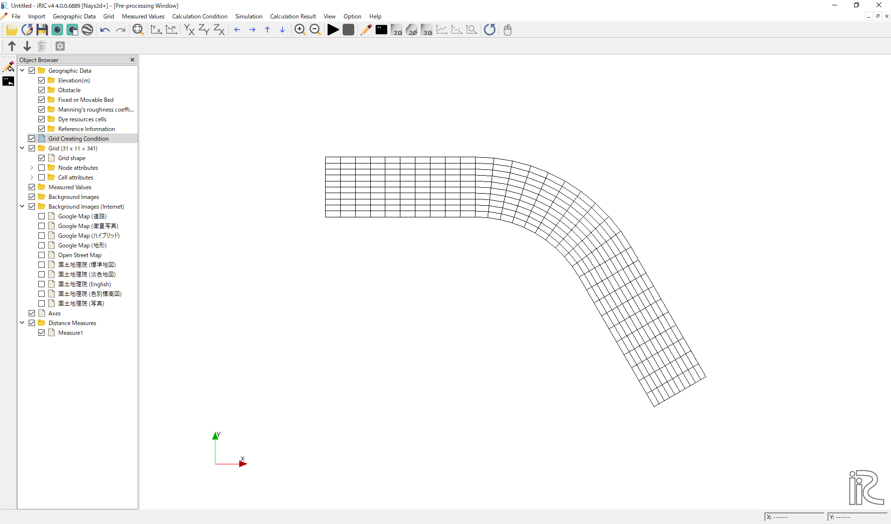
Figure 11 :Computational Grid Completed
For the confirmation of mapping, add tick marks to “grid”, “node attributes”, and “Elevation(m)” in the object browser. A channle with a simple curved channel with straight channels upstream and downstream with parabolic shape section as: numref:01_koushi_5 is shown.
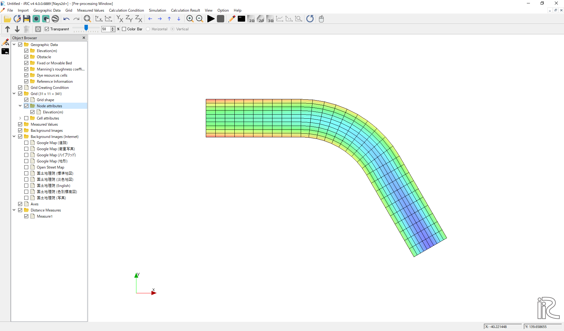
Figure 12 :Confirmation of the mapping result
Set Calculation Condition
From the main menu, select “Calculation conditions”-> “Settings” from the menu bar.
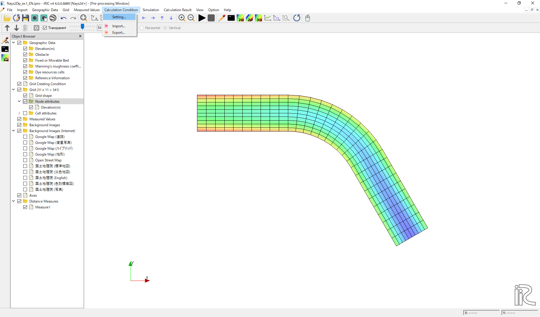
Figure 13 :Calculation conditions setting
Then the calculation condition setting window Figure 14 is displayed.
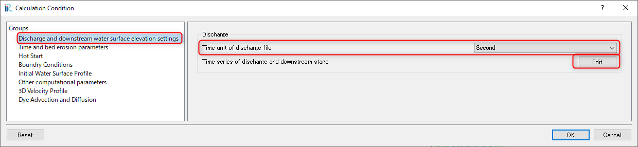
Figure 14 :Calculation condition
Click [Edit] in Figure 14 , and input dischrge hydrograph as shown in Figure 15 . Then click [OK].
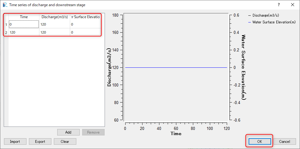
Figure 15 :Time series of discharge input
Select [Time and bed erosion parameters] and set values as shown in Figure 16 .
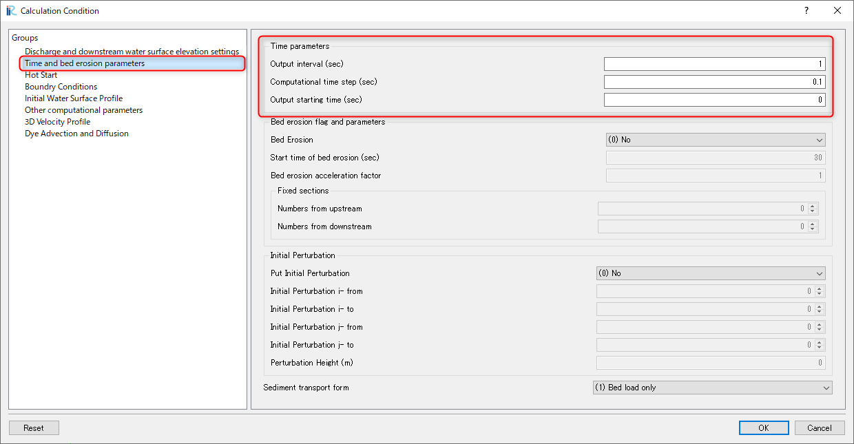
Figure 16 :Setting of time and bed erosion parameters
Select [Other computational parameters] and set values as shown in Figure 17 .
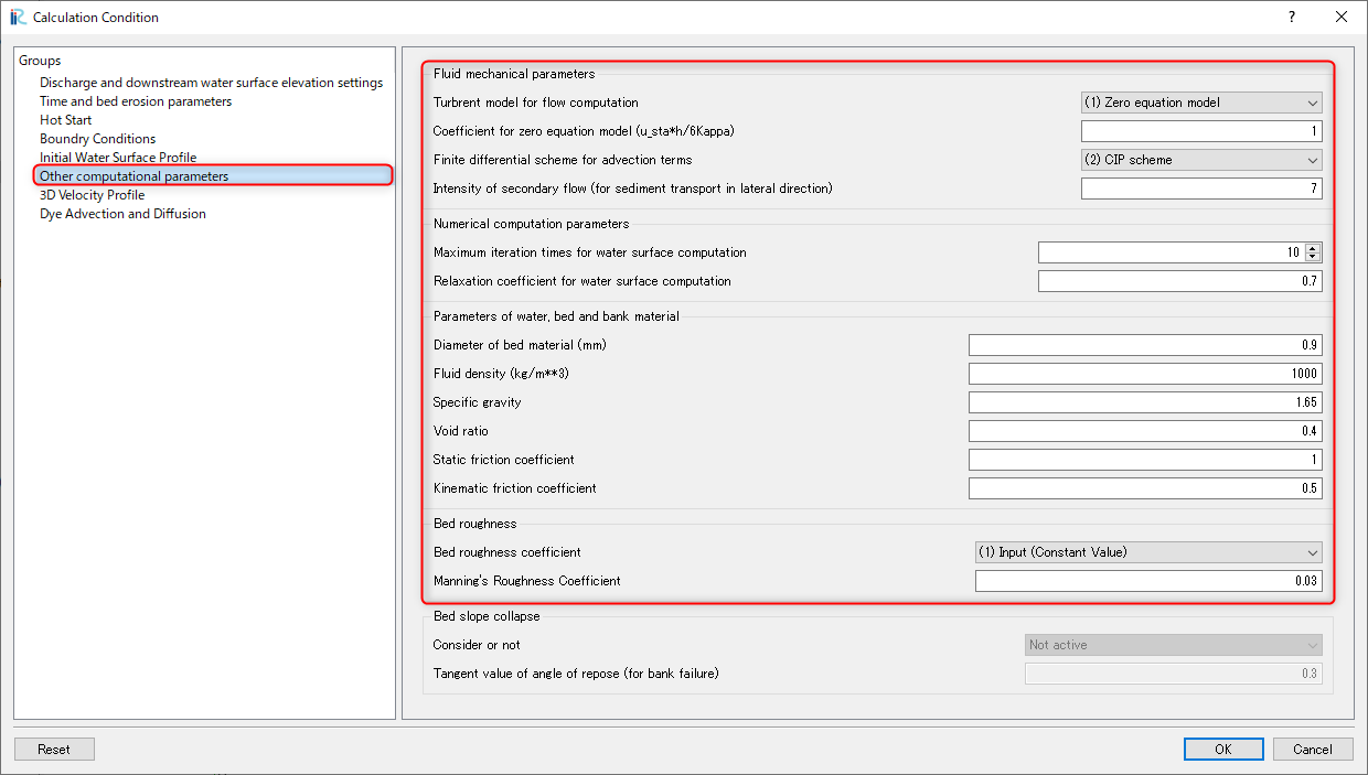
Figure 17 :Setting of Other computational parameters
Select [3D Velocity Profile] and set values as shown in Figure 18 .
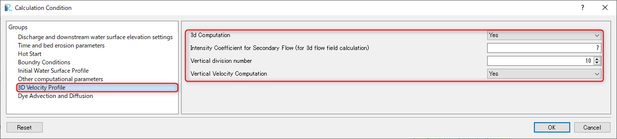
Figure 18 :Setting of 3D velocity profile parameters
Finally, click [OK] and finish condition setting.
Launch Computation
From the main menu bar, select [Simulation],[Run]. Then if you are asked, [This simulation already has results …] as Figure 19 , just reply [OK] to continue.
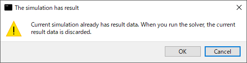
Figure 19 :Warning message(1)
Then you are asked […. Do you want to save?] as Figure 20 . Answer [Yes] or [No] depends on which you want, and the simulation starts as Figure 21
Figure 20 :Warning message(2)
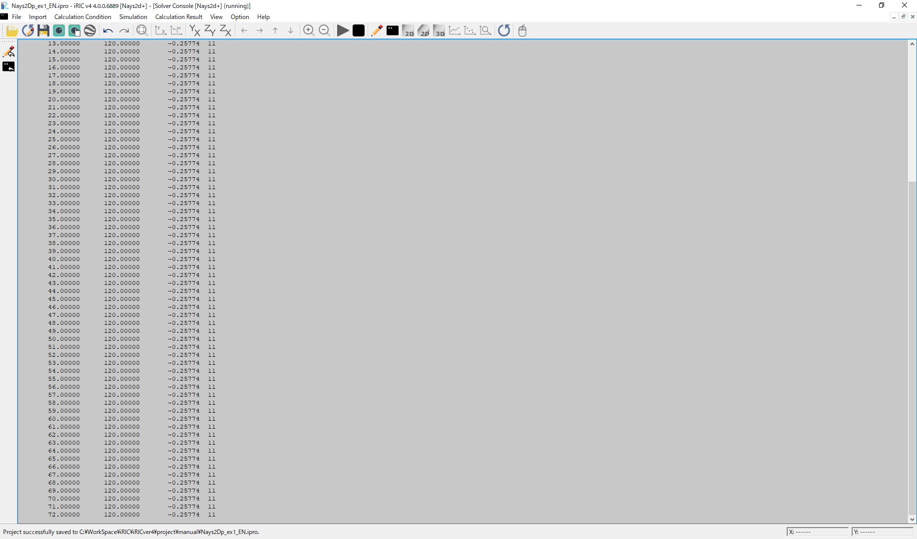
Figure 21 :Simulation
When the simulation finished. A message [The solver finished calculation] appears as Figure 21. Click [OK] and the simulation will finish.
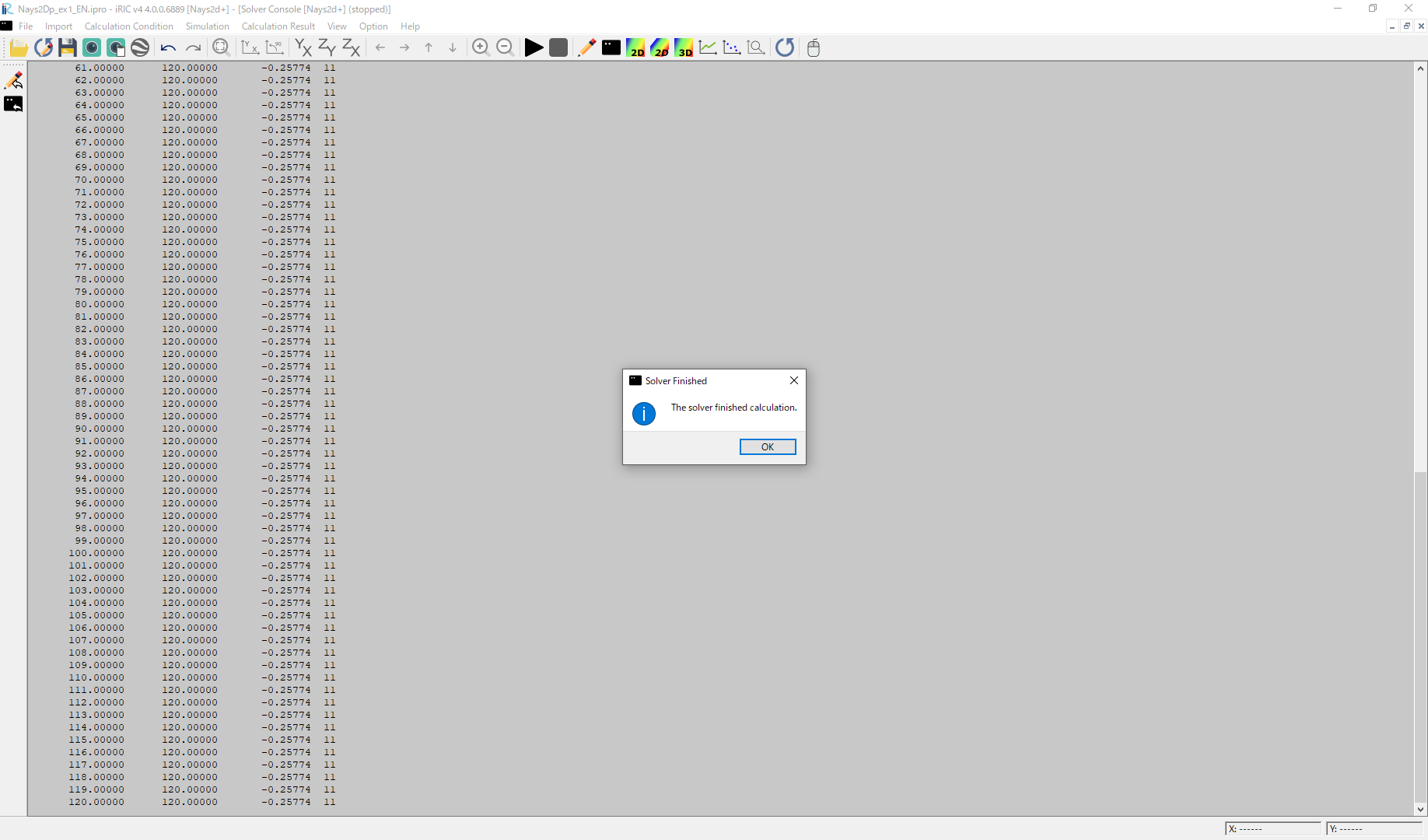
Figure 22 :Simulation finished
Display Computational Results
After the companion finished, form the main menu, by selecting [Calculation Results] and [Open new 2D Post-Processing Window], a new Window appears as Figure 23 .
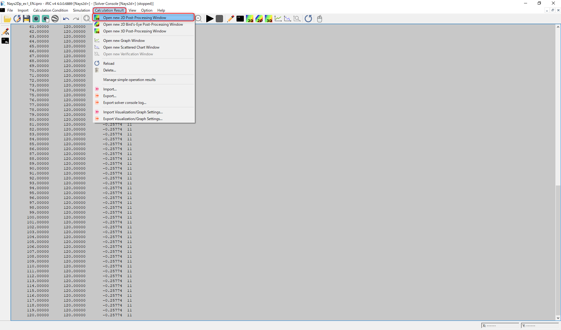
Figure 23 :2D Post-Processing Window
With holding down the “Ctrl” button and the right mouse button, you can move around the object by moving the mouse up/down/left/right. It can also be enlarged and shrank by turning the mouse center diamond as, Figure 24 .
Figure 24 : Moving and resizing of the object image
Depth
In the object browser, put the check marks in “Scalar (node)” and “Depth[m]”, right-click and select “Properties”. The “Scalar Setting” window Figure 25 appears.
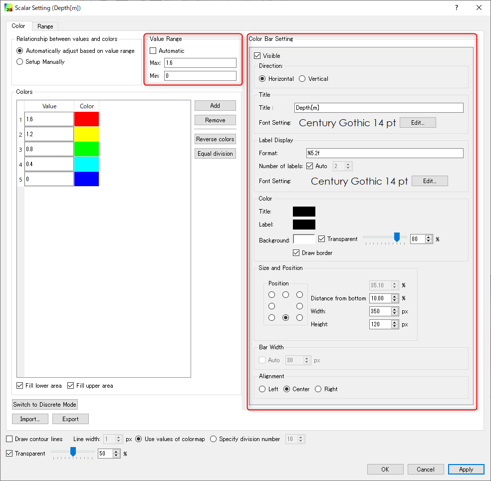
Figure 25 :Scalar Setting
Set the values as shown in Figure 25, and click [OK], then Figure 26 appears.
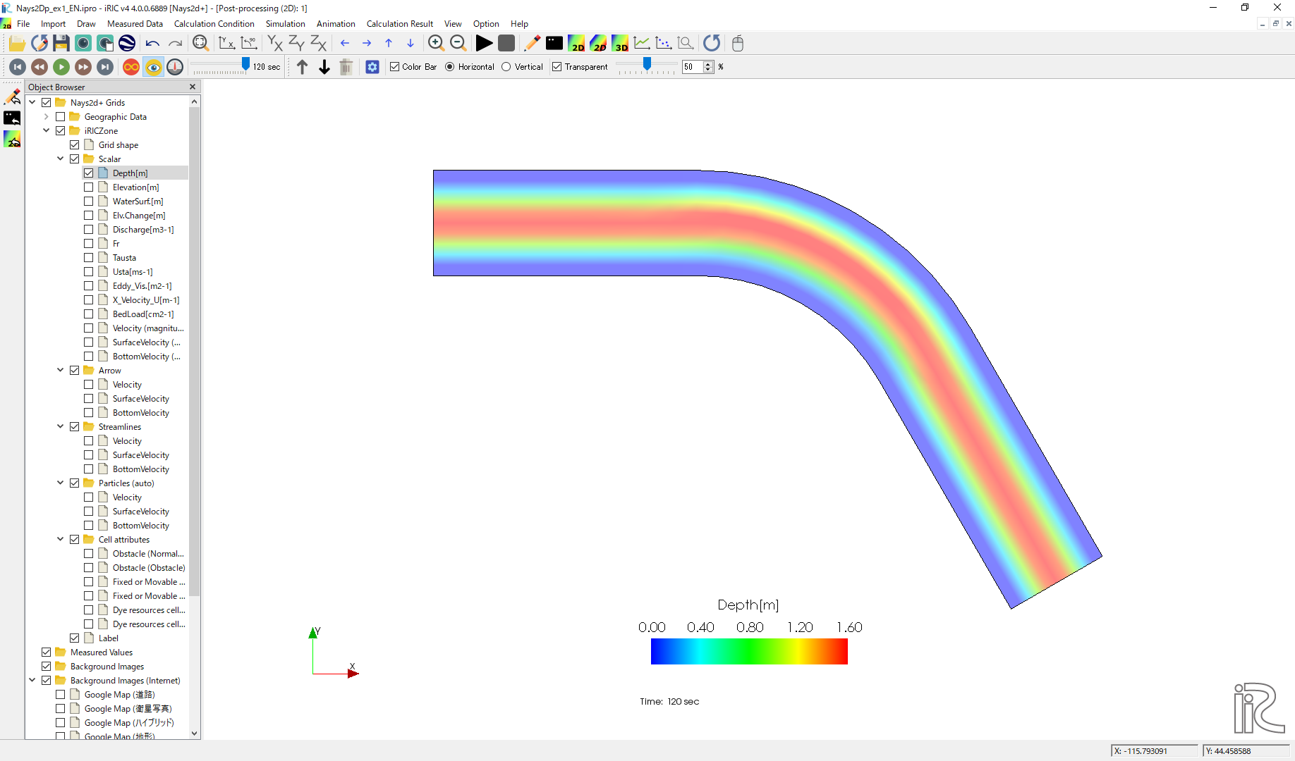
Figure 26 : Depth Plot
Velocity Vectors
In the object browser, put the check marks in “Arrow” and “Velocity”, right-click and select “Properties”. The “Arrow Setting” window Figure 27 appears. Set the values as Figure 27, and click [OK].
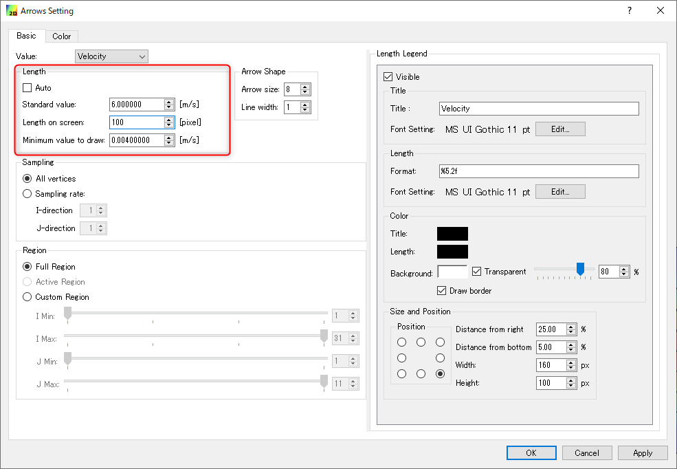
Figure 27 :Arrow Setting
Figure 28 shows the depth-averaged velocity vectors.

Figure 28 :Depth Averaged Velocity Vectors
In Figure 28, you can select “Surface Velocity” and “Bottom Velocity” by chekking each box in “Arrow” group.
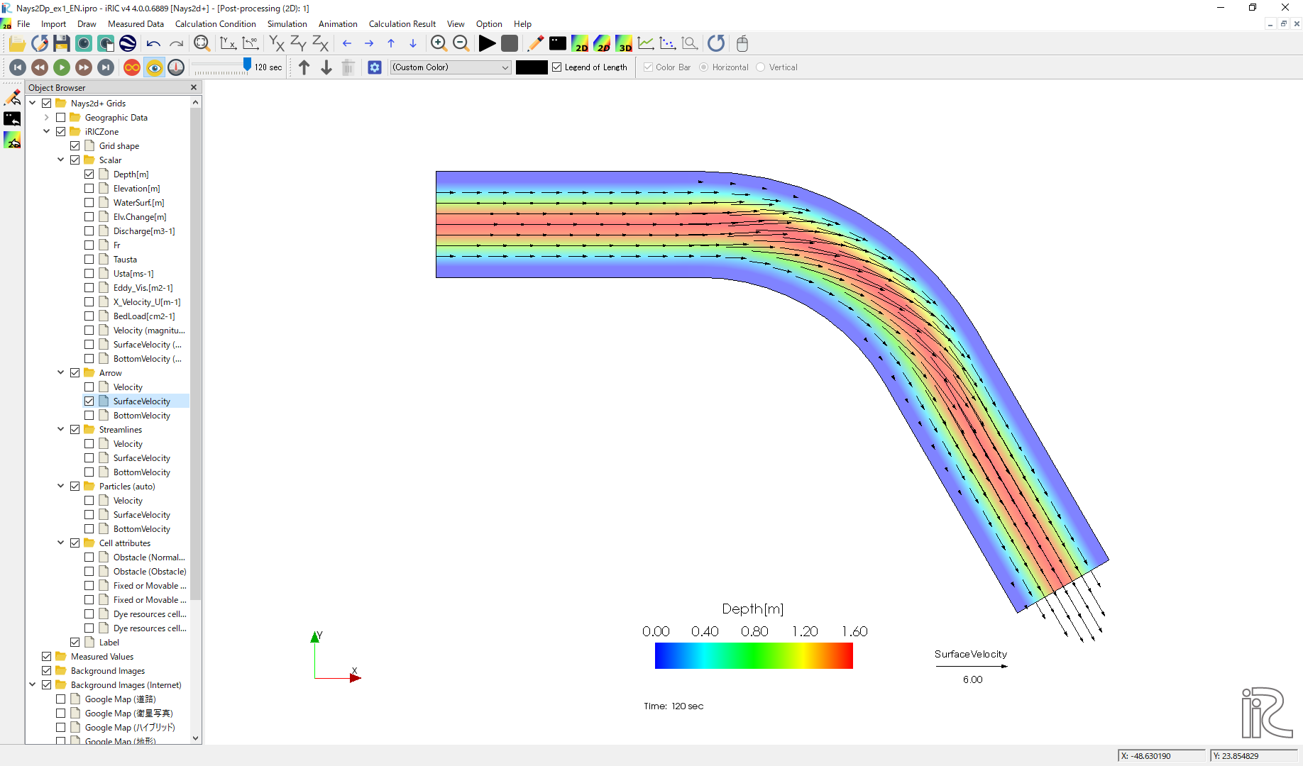
Figure 29 : Surface Velocity Vectors
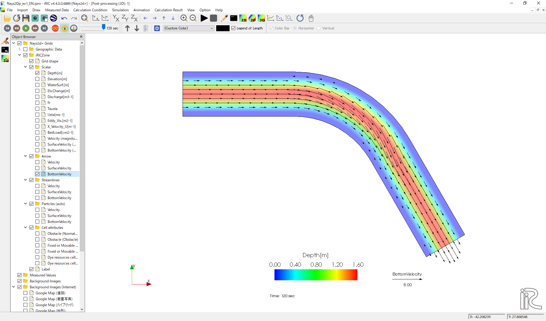
Figure 30 : Bottom Velocity Vectors
It is obvious that, because of the secondly flow, the depth averaged velocity vectors are parallel to the channel banks, the surface velocity vectors are heading to outer bank, and the bottom velocity vectors are heading inner bank.
Stream Lines
Uncheck the box by “Arrow” in the Object Browser and check a box by “Streamline”. By checking “Velocity”, the streamlines following the depth averaged flow velocity” Figure 31 will be displayed. By checking “Surface Velocity”, the streamline following the surface velocity” Figure 32 will be displayed. By checking “Bottom Velocity”, the streamline following the bottom velocity ne: numref:01_kekka_11 will be displayed.
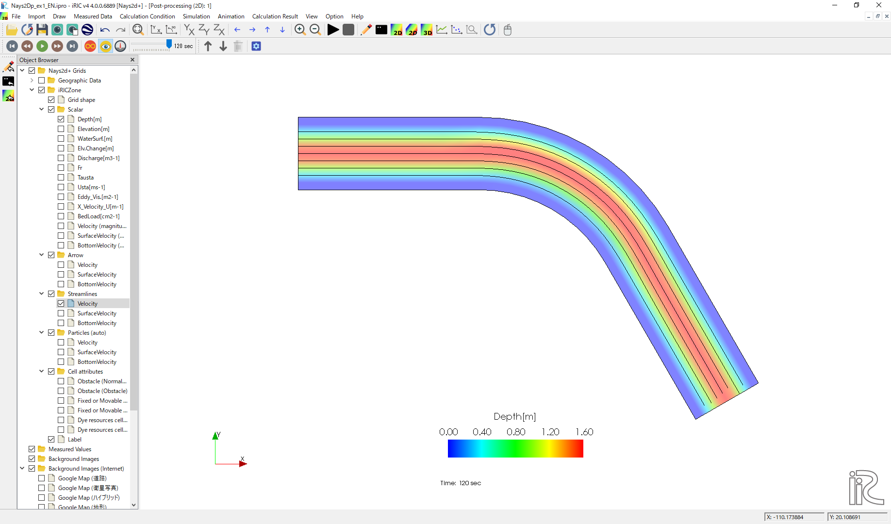
Figure 31 :Streamlines by depth averaged velocity
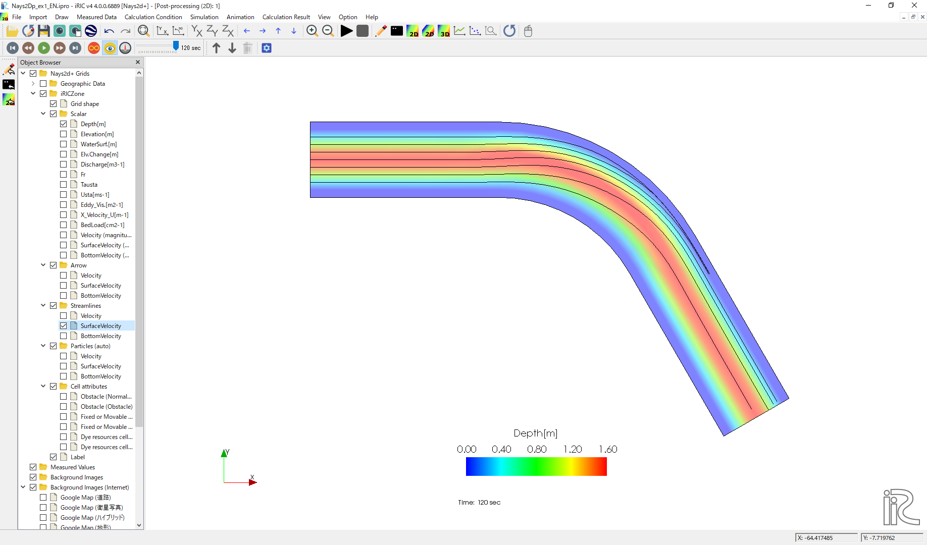
Figure 32 :Streamlines by surface velocity
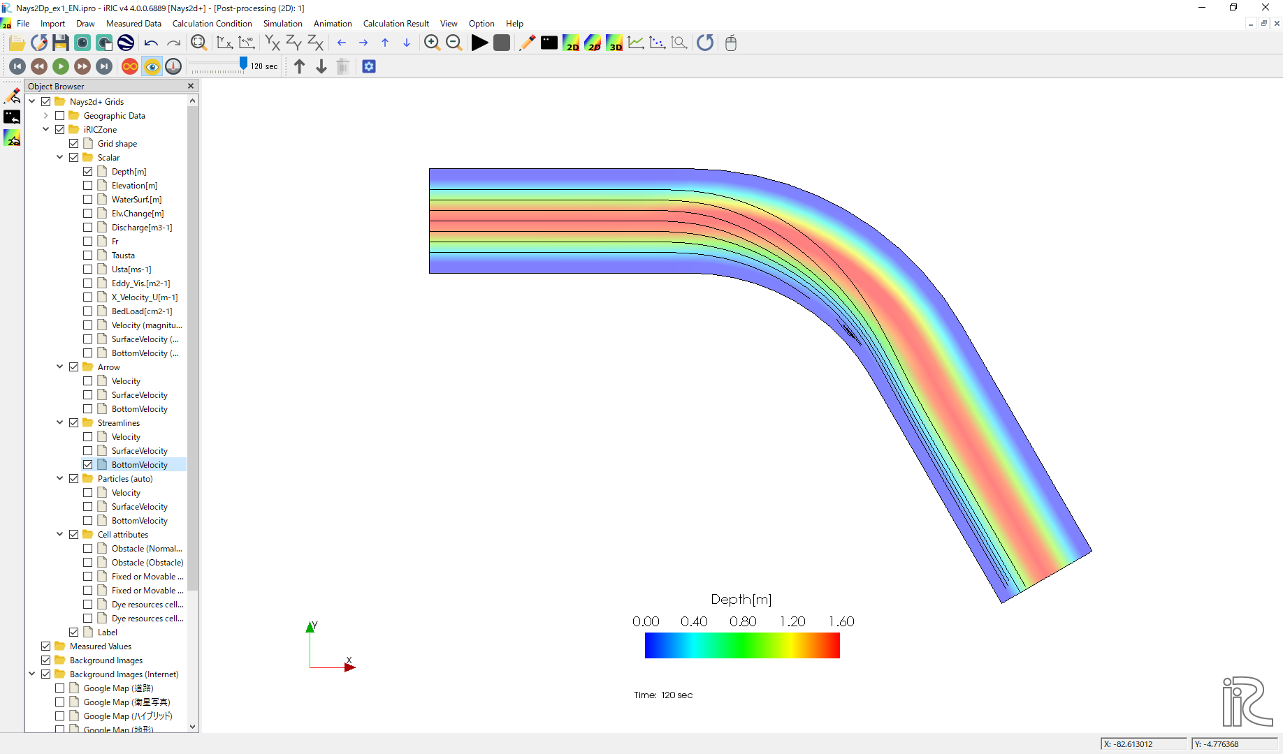
Figure 33 :Streamlines by bottom velocities
The effect of the secondary flow is clearly shown.