[Example 4] Flow in a real river(single cross section)
Select Solver
In the [Select Solver] window, Figure 84 , select [Nays2d+] and click [OK].
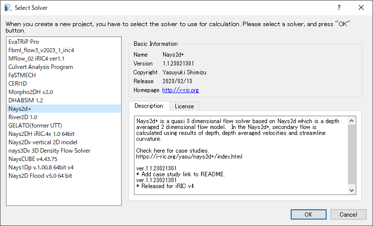
Figure 84 : Select Solver
Importing River Survey Data
In the window, Figure 85, select [Import], [Geographic Data], [Elevation(m)]
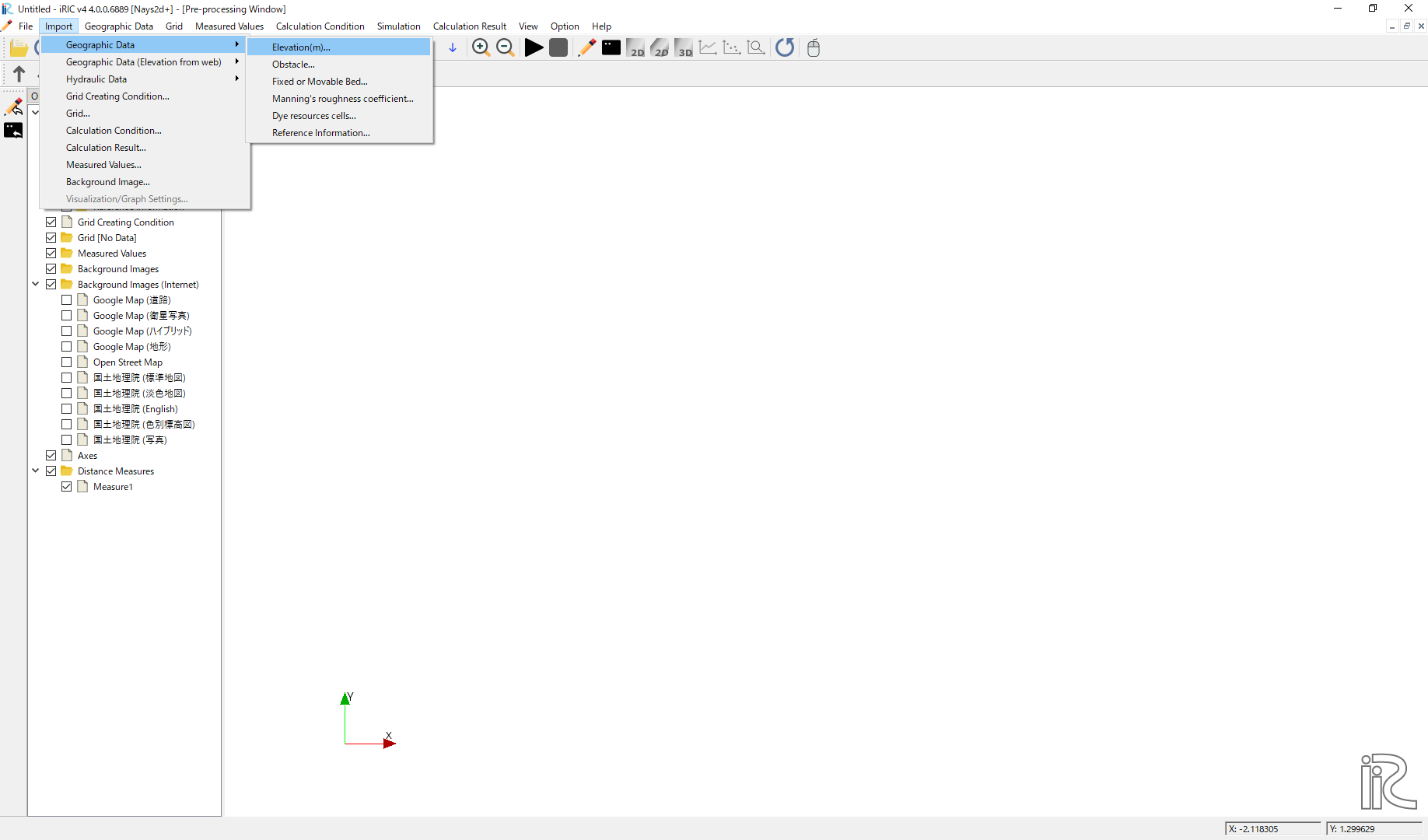
Figure 85 : Import river geographic data
Chose [single.riv] in the window, Figure 86 and open. The cross sectional survey data “single.riv” can be downloaded from, https://i-ric.org/yasu/fw/rivfiles/single.riv
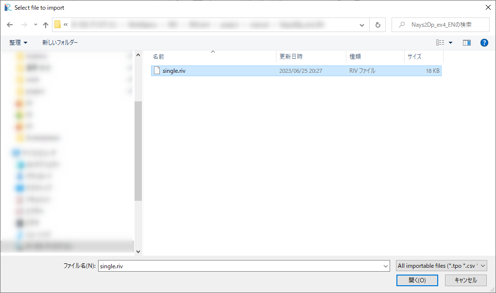
Figure 86 : Select File
A message window may appear telling “Problems Fund i Data” as Figure 87 ,but just click [OK]
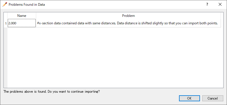
Figure 87 : Prblem Fund
Select [Middle point of left and right bank] in the [River Survey Data Import Setting] window as Figure 88 , and click [OK]
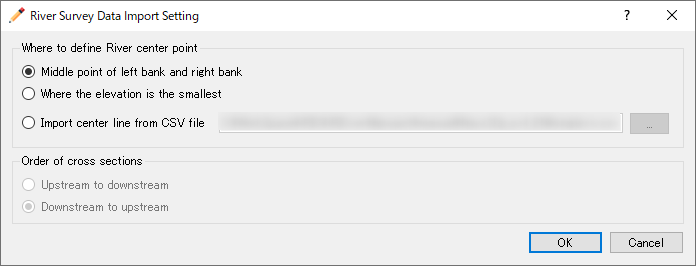
Figure 88 : River Survay Data Import Setting
Figure 89 riv file import complete.
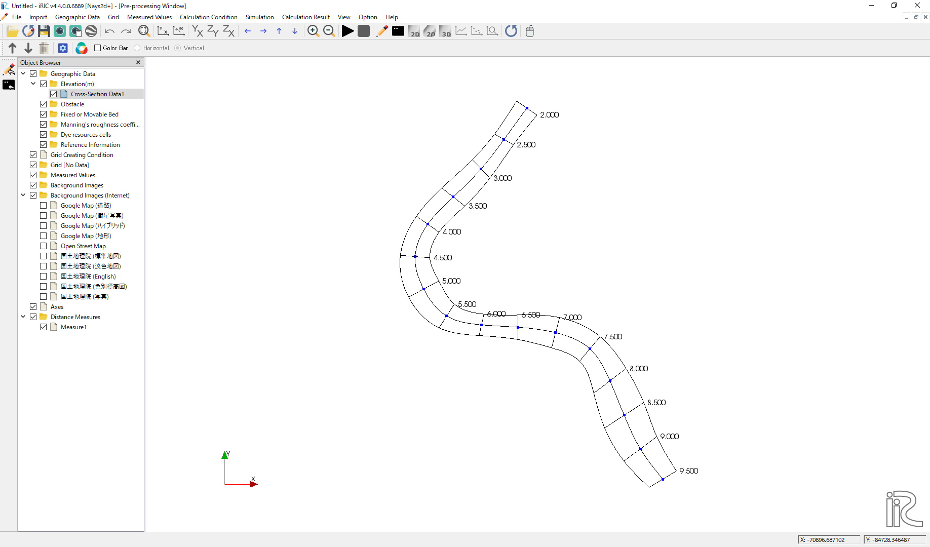
Figure 89 : Import Complete
Grid Generation Conditions
From the main menu, select [Grid] and [Select Algorithm to Create Grid] as, Figure 90
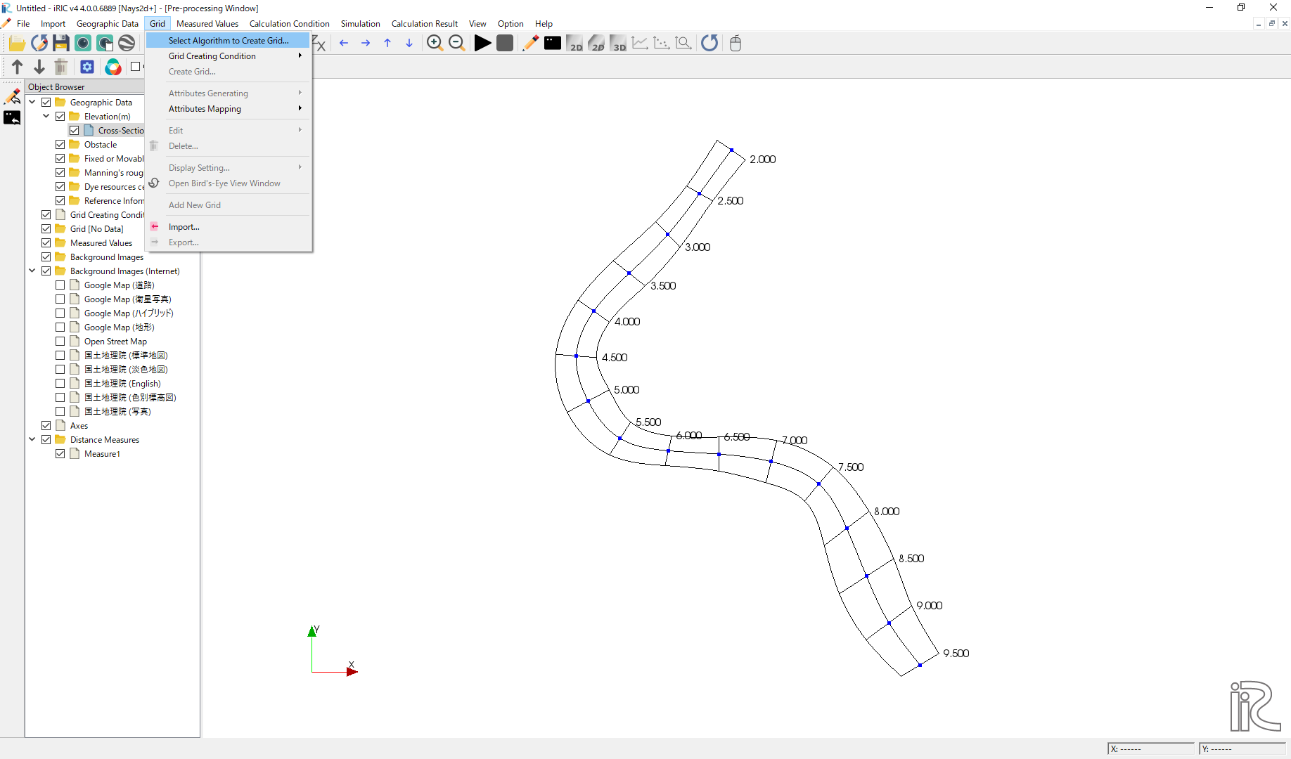
Figure 90 : Select Algorithm to Create Grid
Select [Create grid from river survey data] from the window, Figure 91 , and click [OK].
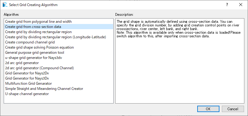
Figure 91 : Create grid from river survey data
As shown in Figure 92 , a channel with cross sections with both ends’ blue circles are displayed.
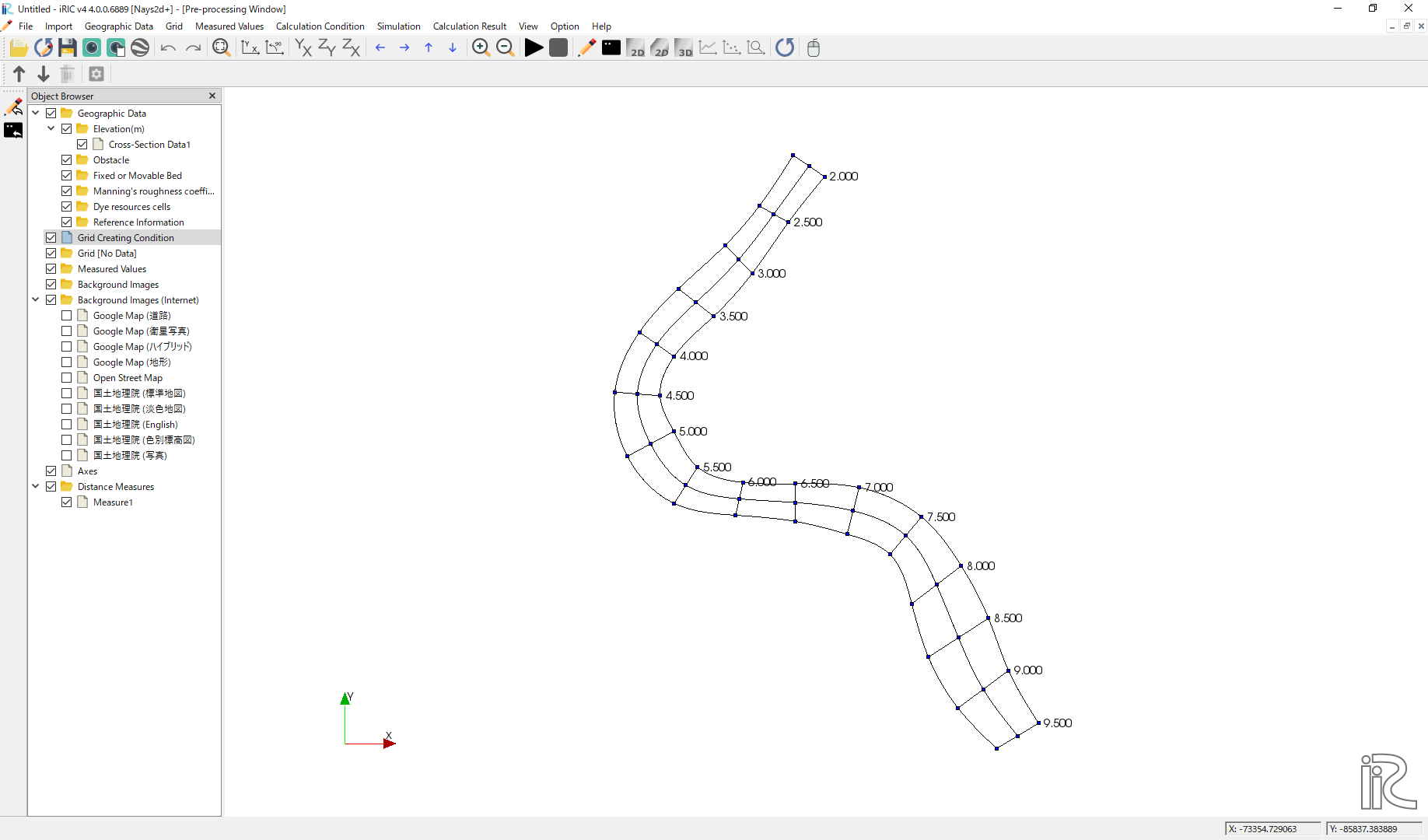
Figure 92 : Setting Grid Create Condition Complete
Grid Generation
Select any side of one of the cross section line, right click, and chose [Add Division Points].
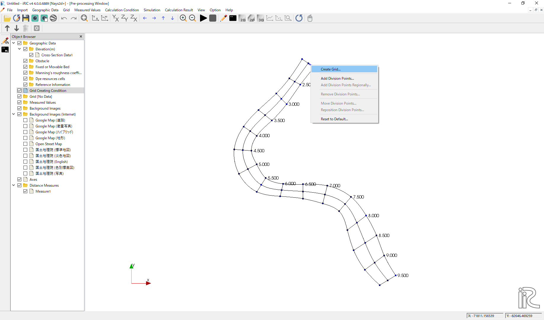
Figure 93 :Add Division Points(1)
Set [Division Number], set [4] in this example, and click [OK] (Figure 94 )
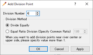
Figure 94 :Add Division Points(2)
Select one of the opposite side of the cross sectional line we selected in Figure 93 , right click, and chose [Add Division Points] (Figure 95 )
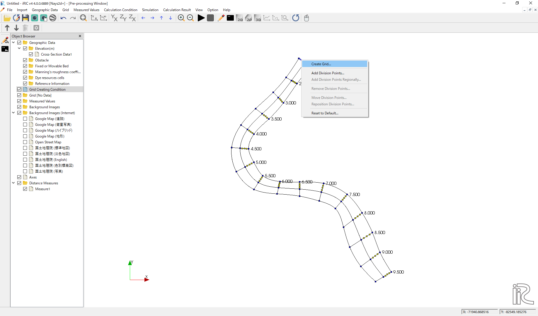
Figure 95 :Add Division Points(3)
Set [Division Number], set [4] as a same number we set in Figure 94 for the symmetry.
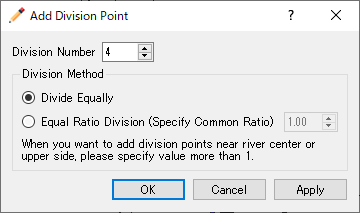
Figure 96 :Add Division Points(4)
Along the channel direction, division points are set all at once. Select [Grid], [Add Division Points Regionally] from the menu bar. ( Figure 97 )
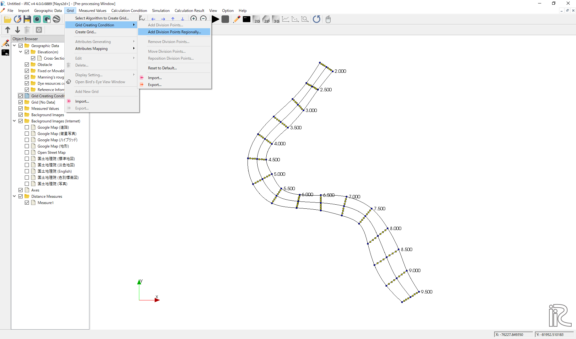
Figure 97 :Add Division Points Regionally(1)
Chose [Specify target distance division points]. set distance [70] in this example, and click [OK].( Figure 98 )
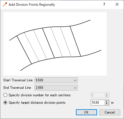
Figure 98 :Add Division Points Regionally(2)
When the setup for division points are completed, a plane map with yellow circle points appears as Figure 99
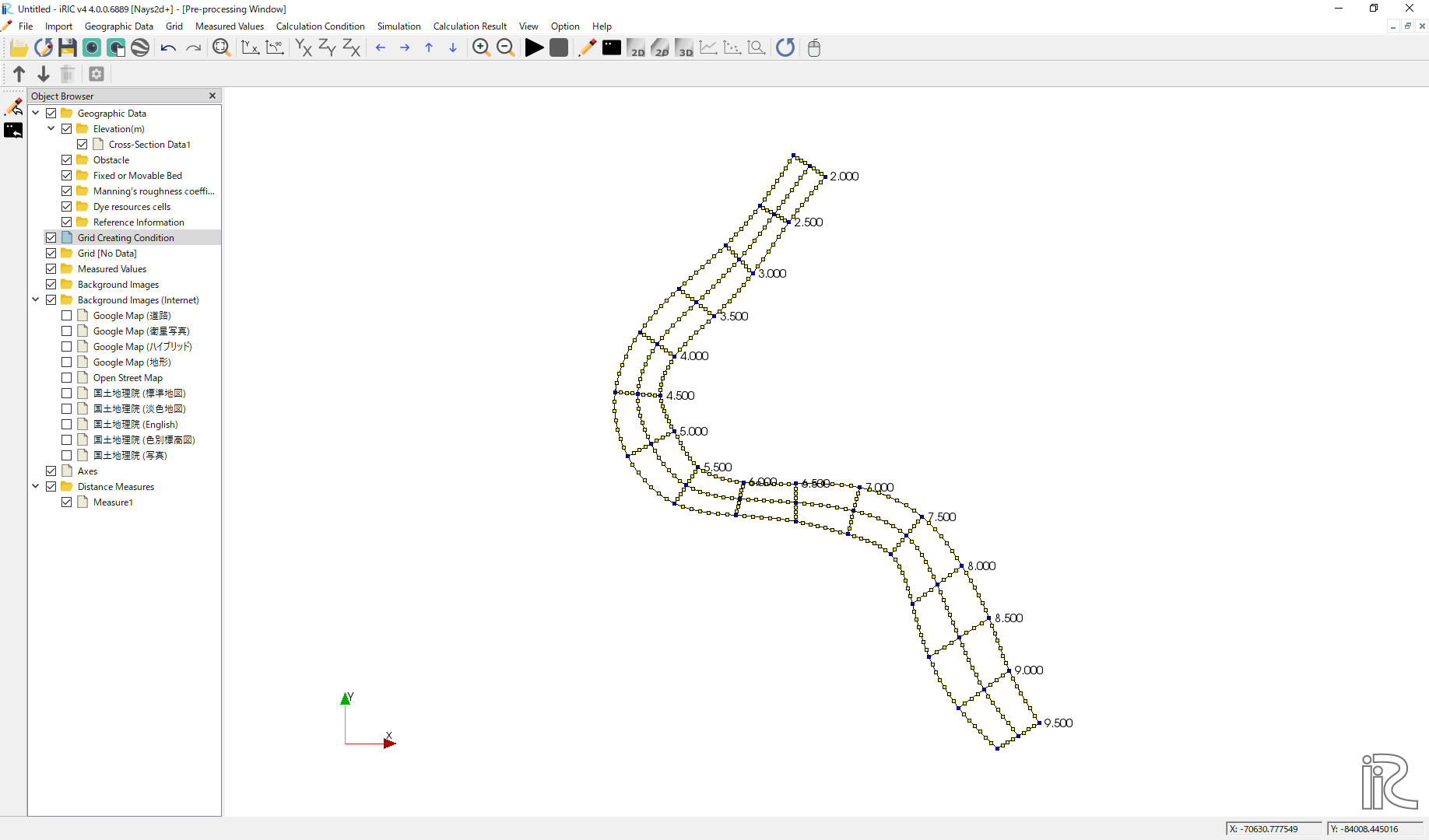
Figure 99 :Set dicision points complete
Select [Grid], [Grid Create] from the menu bar.( Figure 100 )
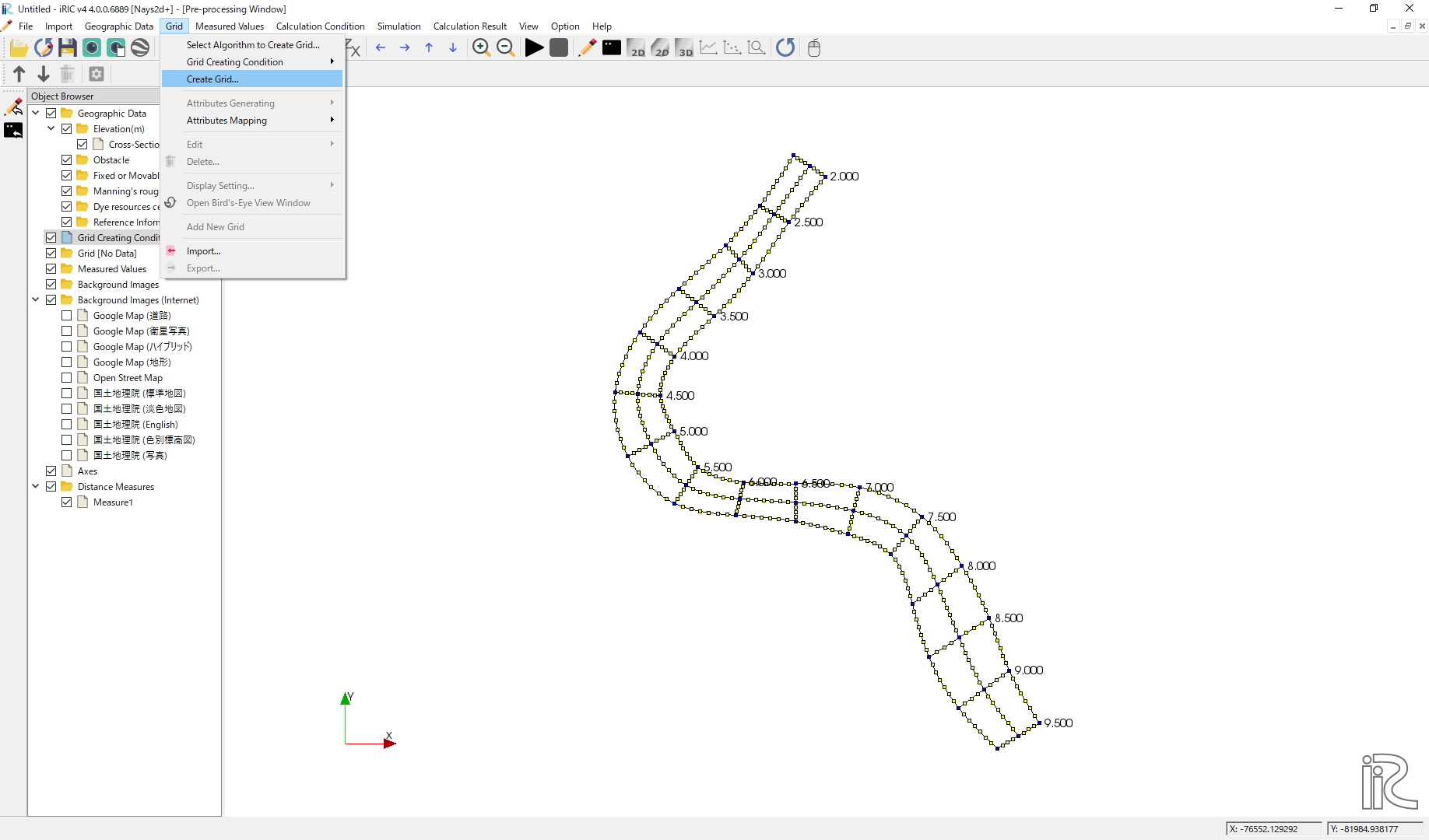
Figure 100 :Grid Create(1)
Confirm the grid generation range painted with blue, and click [OK].
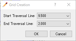
Figure 101 :Grid Create(2)
Answer [Yes] when you asked [Do you want to map?] as Figure 102
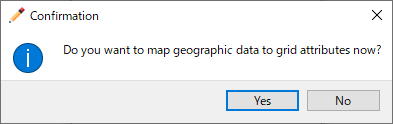
Figure 102 :Mapping?
Completed grid is shown as Figure 103
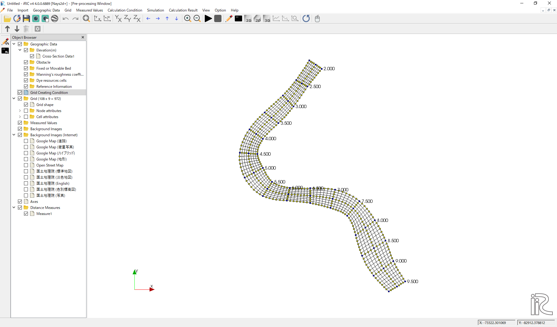
Figure 103 :Grid Generation Complete
Bed configuration and channel shape can be confirmed by putting checking marks at, [Grid], [Node attributes] and [Elevation (m)]. ( Figure 104 )
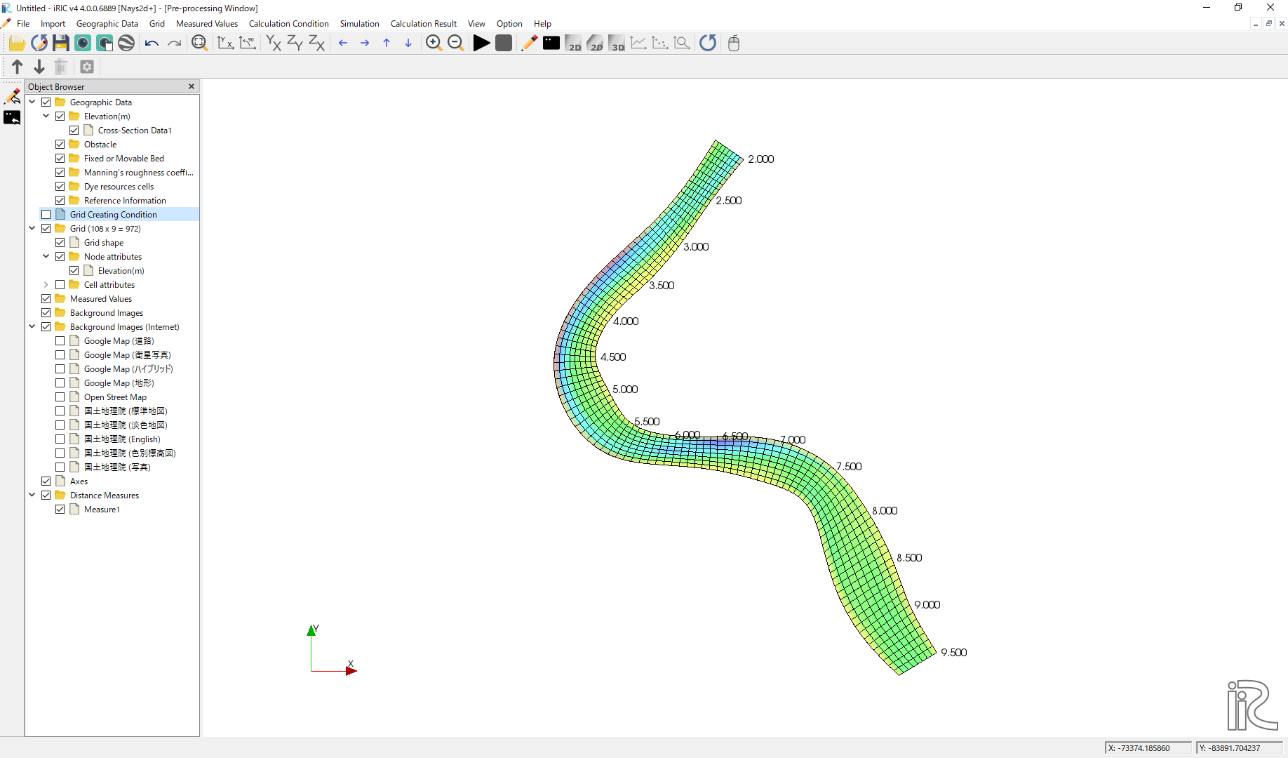
Figure 104 :Confirmtion of the Mapping Result
Computational Condition
Select [Calculation Condition] and [Setting] from the min menu as Figure 105 .
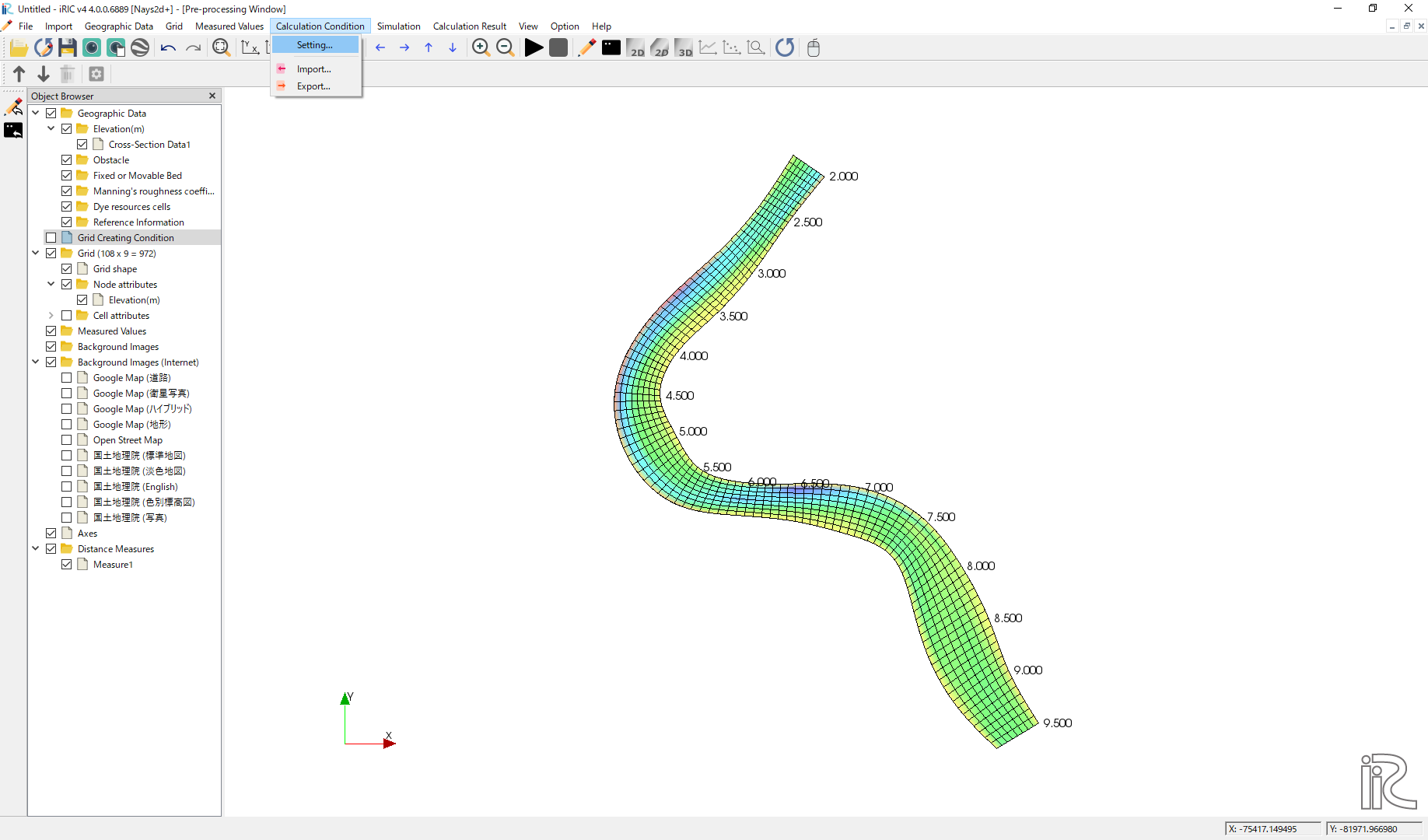
Figure 105 :Setting Compitational Condition
Set [Time unit of discharge] as [Hour] and click [Edit], ( Figure 106 )
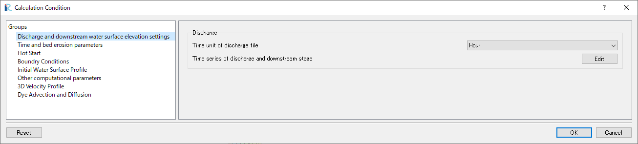
Figure 106 :Discharge Condition
Set discharge hydrography as Figure 107, constant for 3 hours with 2,000 qms, and click [OK].
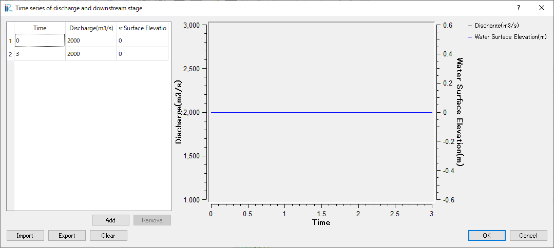
Figure 107 :Input Discharge(2)
Set [Time and bed erosion condition] as Figure 108 .
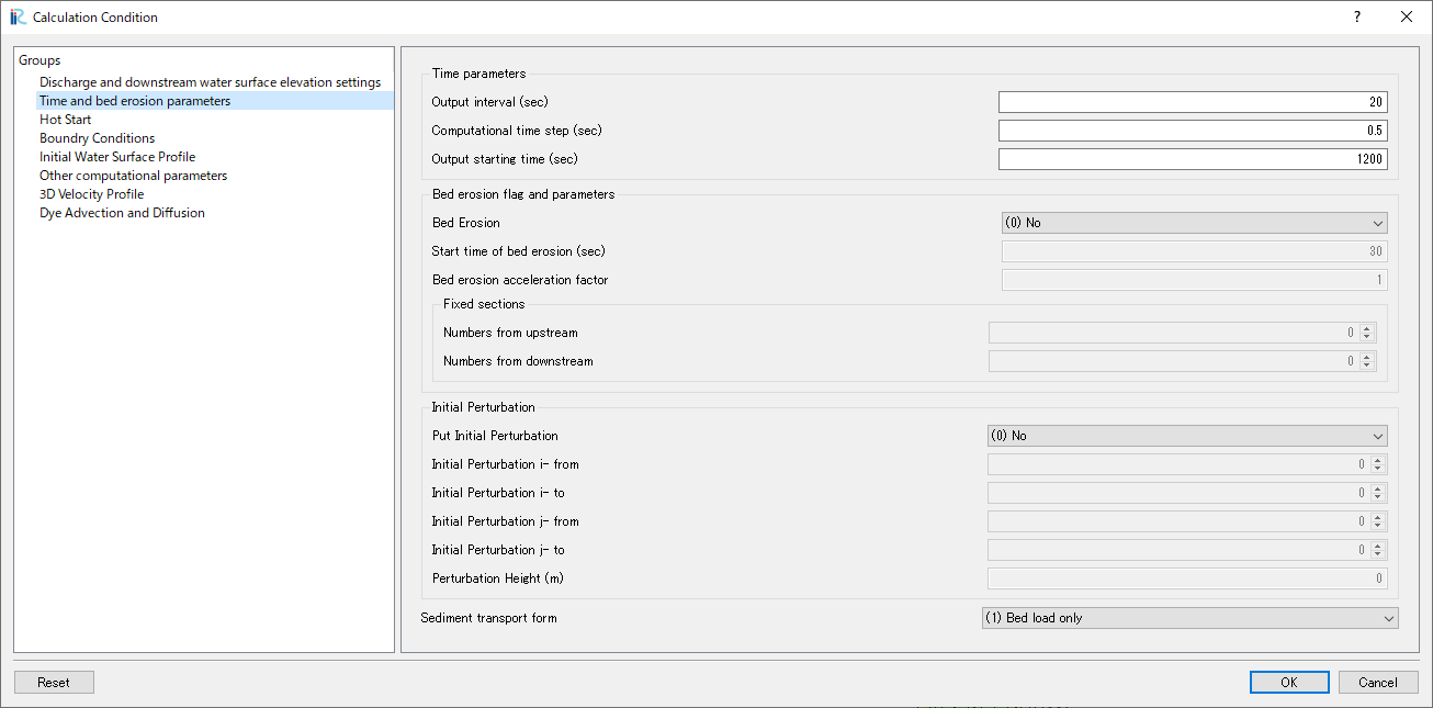
Figure 108 :Time and bed erosion condition
Set [Boundary Conditions] as Figure 109 .
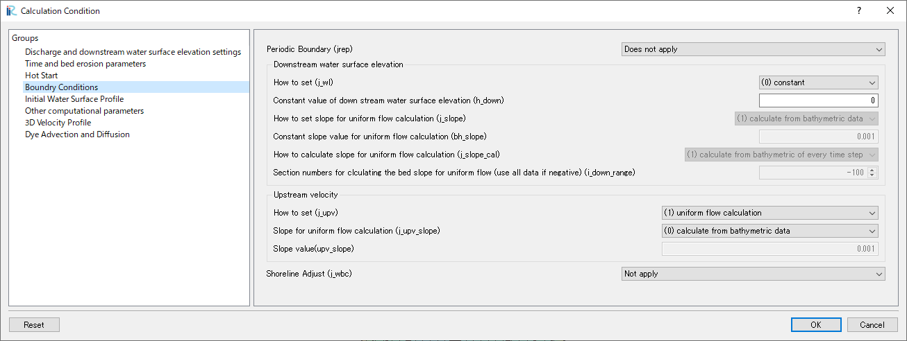
Figure 109 :Boundary Conditions
Set [Initial Water Surface Profile] as Figure 110 .
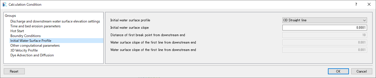
Figure 110 :Initial Water Surface Profile
Set [Other computational parameters] as Figure 111 .
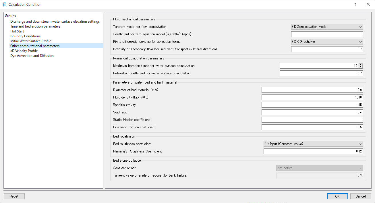
Figure 111 :Other computational parameters
Set “3D Velocity Profile” as shown in the figure Figure 112 , and click [OK] to exit.
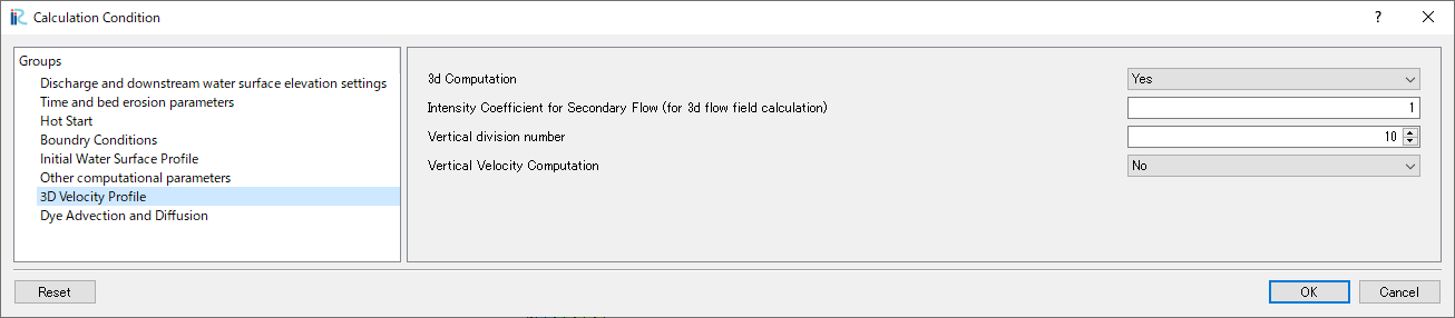
Figure 112 :3D Velocity Profile Settings
Launch Computation
From the menu bar, select [Simulation] and [Run].
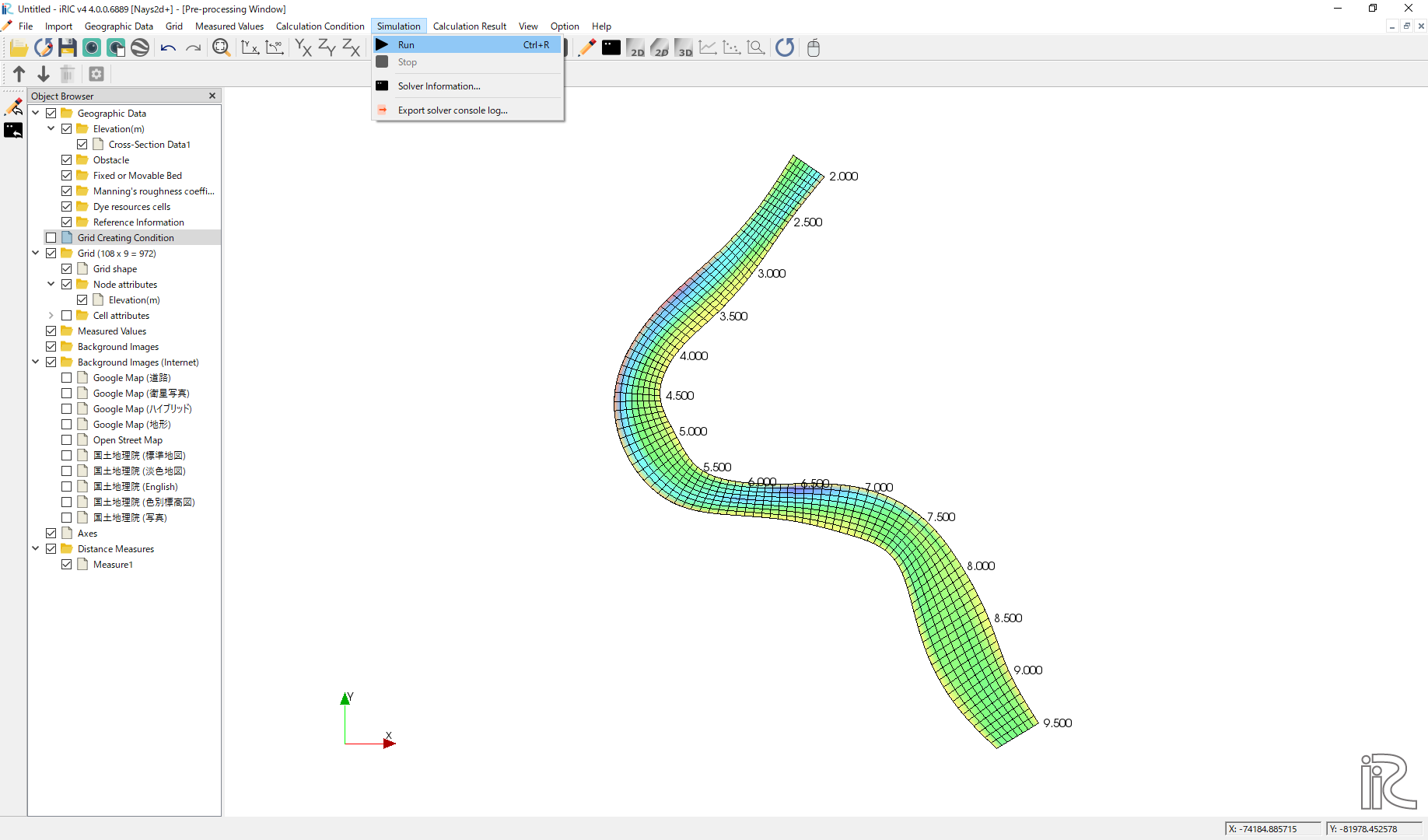
Figure 113 :Launch Simulation(1)
Answer [Yes(Y)] when you asked [Save the project?] as Figure 114
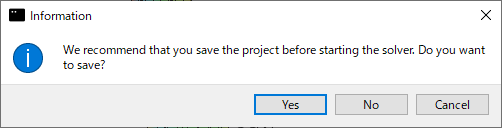
Figure 114 :Launch Simulation(2)
Simulation starts. Figure 115
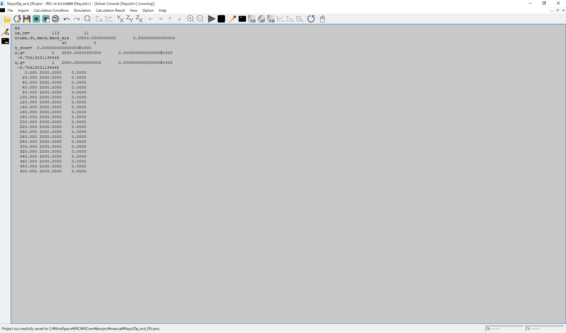
Figure 115 :Launch Simulation(3)
Click [OK] when the message [The solver finished calculation] as Figure 116
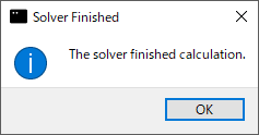
Figure 116 :Calculation finished
Display Computational Results
After the companion finished, form the main menu, by selecting [Calculation Results] and [Open new 2D Post-Processing Window], a new Window appears as Figure 117 .
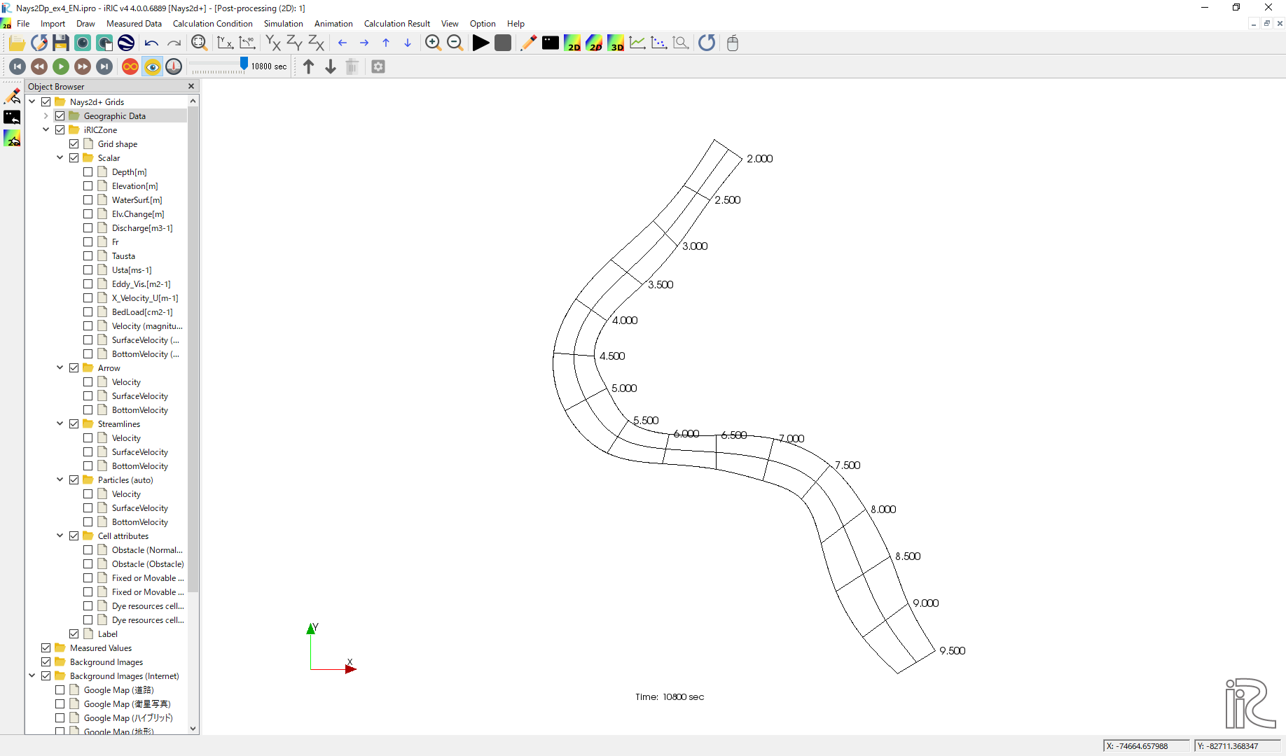
Figure 117 :2D Post-Process Window
Depth
n the object browser, put the check marks in “Scalar (node)” and “Depth[m]”, right-click and select “Properties”. The “Scalar Setting” window Figure 118 appears.
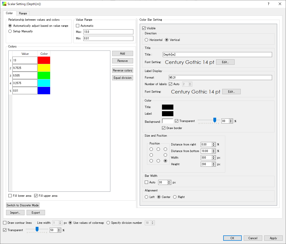
Figure 118 :Scalar Setting
Set the values as shown in Figure 118, and click [OK], then Figure 119 appears.
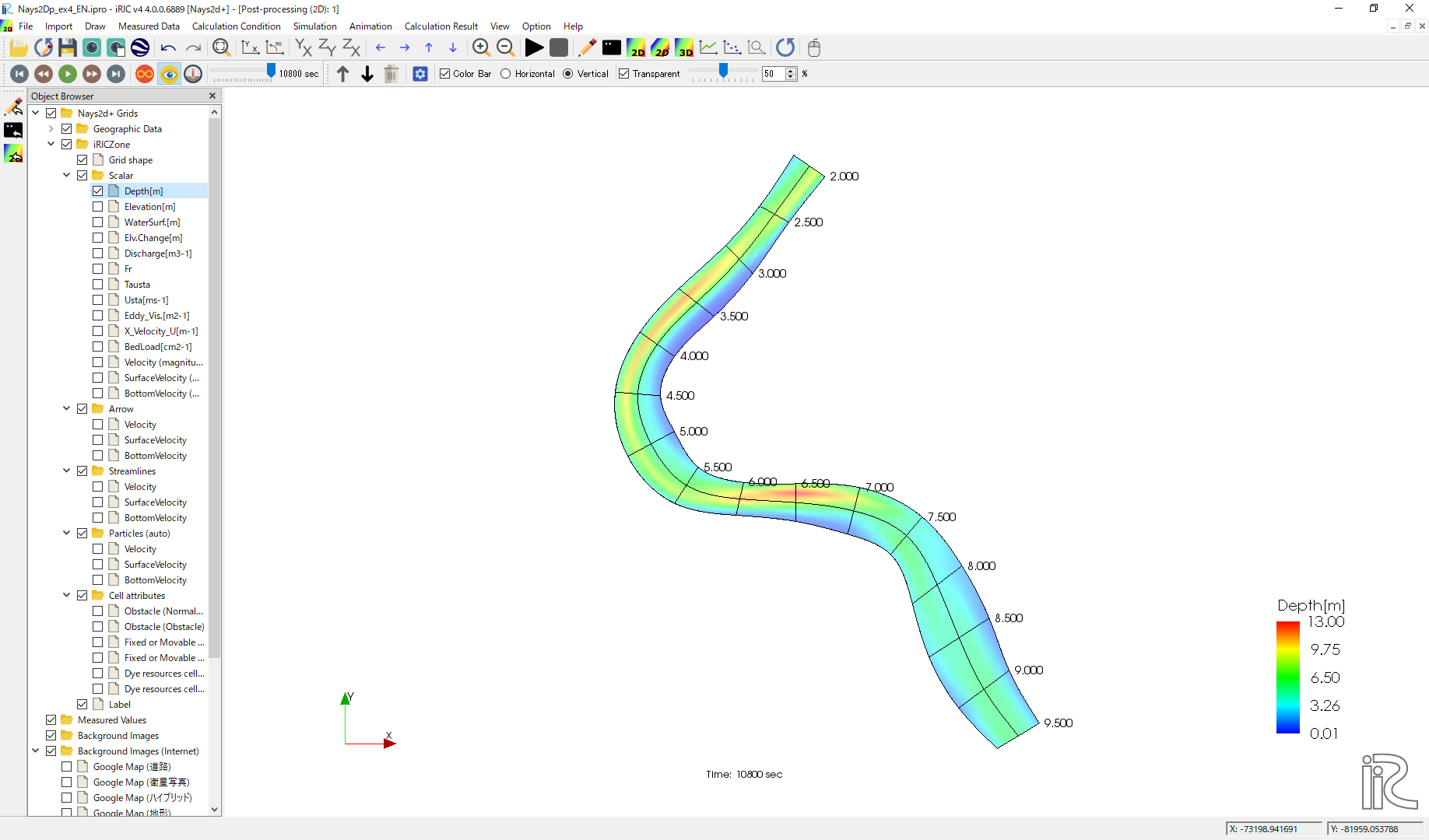
Figure 119 : Depth Plot
Display Background Image
Select from the main menu, [File]->[Property] ( Figure 120 )
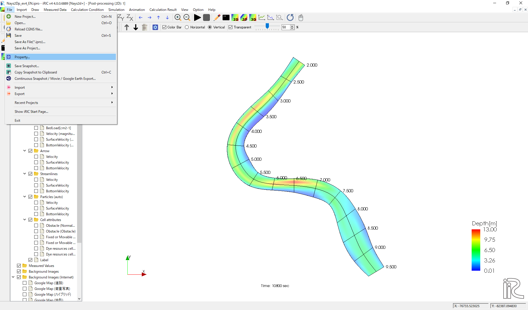
Figure 120 :Select Property
From the “Project Property” window, click [Edit] at [Coordinate System] .. _04_haikei_02:
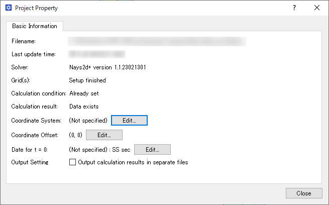
Figure 121 :Edit Coordinate System Setting
Input “Japan” in the [Search] window, and chose the one with “XII” from the items with [EPSG:….] as Figure 122 . See more detail on coordinate system of Japan at http://www.gsi.go.jp/sokuchikijun/jpc.html
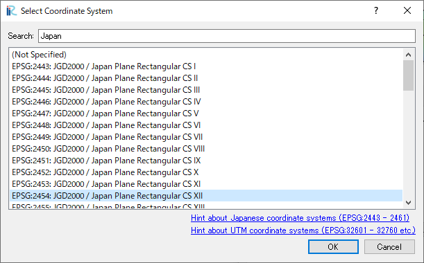
Figure 122 :Select Coordinate System
Click [Close] of [Project Property] window of Figure 123
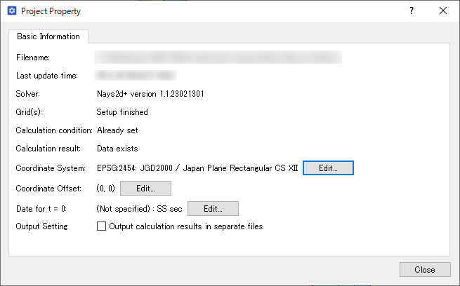
Figure 123 :Close Property Window
Put a check mark in a box in front of [Background Images(Internet)] and one of the items listed below, e.g., [Google Map (Sattelite Image)] as Figure 124
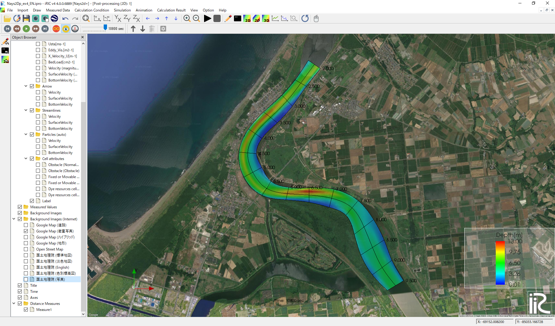
Figure 124 :Background Image Import Complete
Velocity Vectors and Streamlines
Since the operation method is the same as the previous section, it will be omitted.
Particle Animations
Put check mark at [Particles] and [Velocity] in the object browser, put time bar back to zero, and push black button, ( Figure 125 ). Particle following the depth averaged velocity starts as Figure 126 .
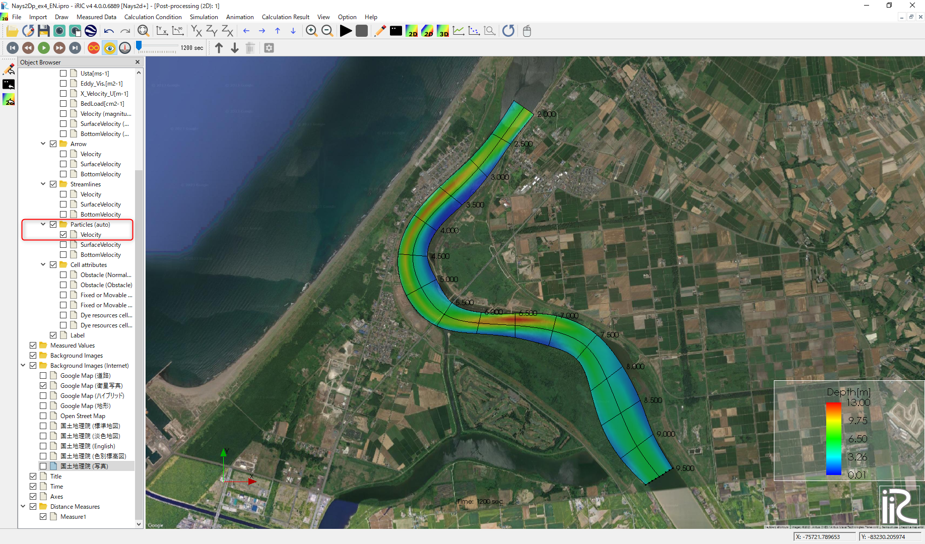
Figure 125 :Particle Animation
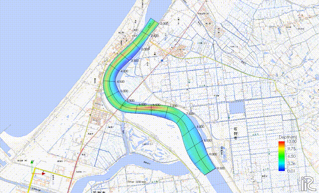
Figure 126 :Particle movement by depth averaged velocity
Make the Particles riding the surface velocity are displayed in red. Put ☑ in “Particle” and “SurfaceVelocity”, right-click on “Particle” and select “Properties” to display “Particle setting screen” Figure 127, so set it as shown in the figure and Click [OK]. Reset the time bar to zero and press the play button to display the particle animation caused by the surface flow of Figure 128.
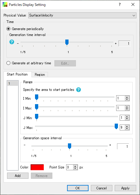
Figure 127 :Particle Setting

Figure 128 :Particle movement by surface velocity
In the same way, the particle flowing animations can be played by checking a box at [Bottom Velocity], respectively.

Figure 129 :Particle movement by bottom velocity